Cormit well/aquifer analytics
What makes a good remote monitoring system for wells/aquifers?
A comprehensive well/aquifer monitoring system should provide detailed insights into well performance, aquifer response, and long-term trends. The table shows the key features that enable effective monitoring and analysis of well/aquifer systems.
Cormit's system delivers all these essential features to provide a complete picture of your well and aquifer performance.
| Function | Desired features | Cormit |
|---|---|---|
| Data acquisition |
| |
| Data storage |
| |
| Data analytics |
| |
| Modelling |
| Future |
Well/aquifer metrics generated by Cormit for a cycling well
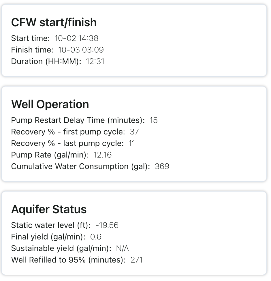
Summary metrics for a CFW (call-for-water) cycle
The table summarizes key metrics generated during a call-for-water cycle, including static water level, recovery percentages, refill times, and sustainable yield calculations.
These metrics provide a comprehensive snapshot of well and aquifer performance during each CFW cycle.
Aquifer performance—during CFW (as pump cycles)
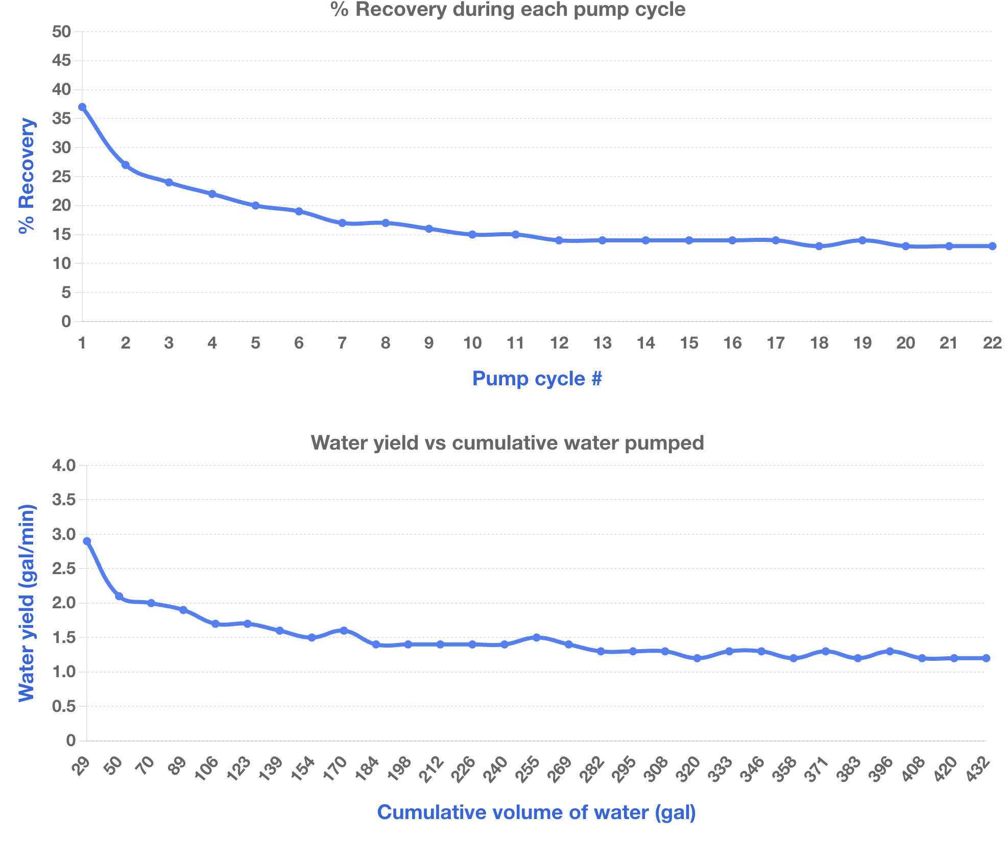
% recovery for each pump cycle:
For each pump cycle during the CFW cycle, the graph shows the amount the well refills expressed as a percentage of the static water level (% recovery). The aquifer's ability to deliver water to the pump declines as the pump continues cycling and then stabilizes if the CFW cycle progresses long enough.
Water yield over CFW cycle:
Well output as a function of cumulative volume of water pumped during a CFW cycle. Generally, the well output drops and then reaches equilibrium level as pumping continues. The water yield after well output stabilizes is the well-level sustainable yield of the well/aquifer system.
These graphs reveal how the aquifer's water delivery capacity changes during extended pumping cycles.
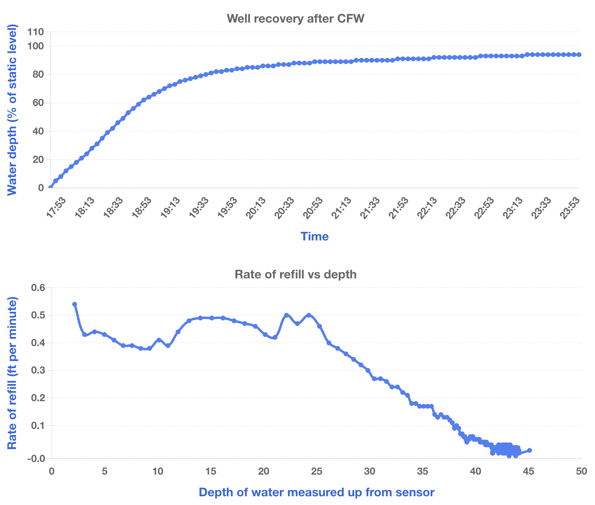
Aquifer performance—post CFW (well refills)
Refill after CFW:
This graph shows the well refilling as a function of time after CFW ends. The refill is measured as the depth of water in the well, expressed as a percentage of the static water level.
If the refill curve starts out linear (straight line), it means the bottom of the aquifer is above the level of the depth sensor in the well. The point at which the initial linear segment ends and rate of refill slows marks the bottom of the aquifer.
Rate of refill as function of depth:
This graph shows the rate at which the well is refilling after a CFW cycle ends as a function of the depth of water in the well.
The rate of refill is measured in units of length per units of time (e.g., inches measured per minute) where "length" is the vertical height of the water in the well. Initially, the rate will be relatively high as the entire well is empty and there is no hydrostatic pressure in the well pushing back against water trying to enter the well. As the well fills with water and the depth goes above the bottom of the aquifer, hydrostatic pressure of the water in the well pushing back against the water trying to enter the well slows the rate of refill.
Post-CFW refill patterns provide critical insights into aquifer structure and transmissivity.
Long term trends
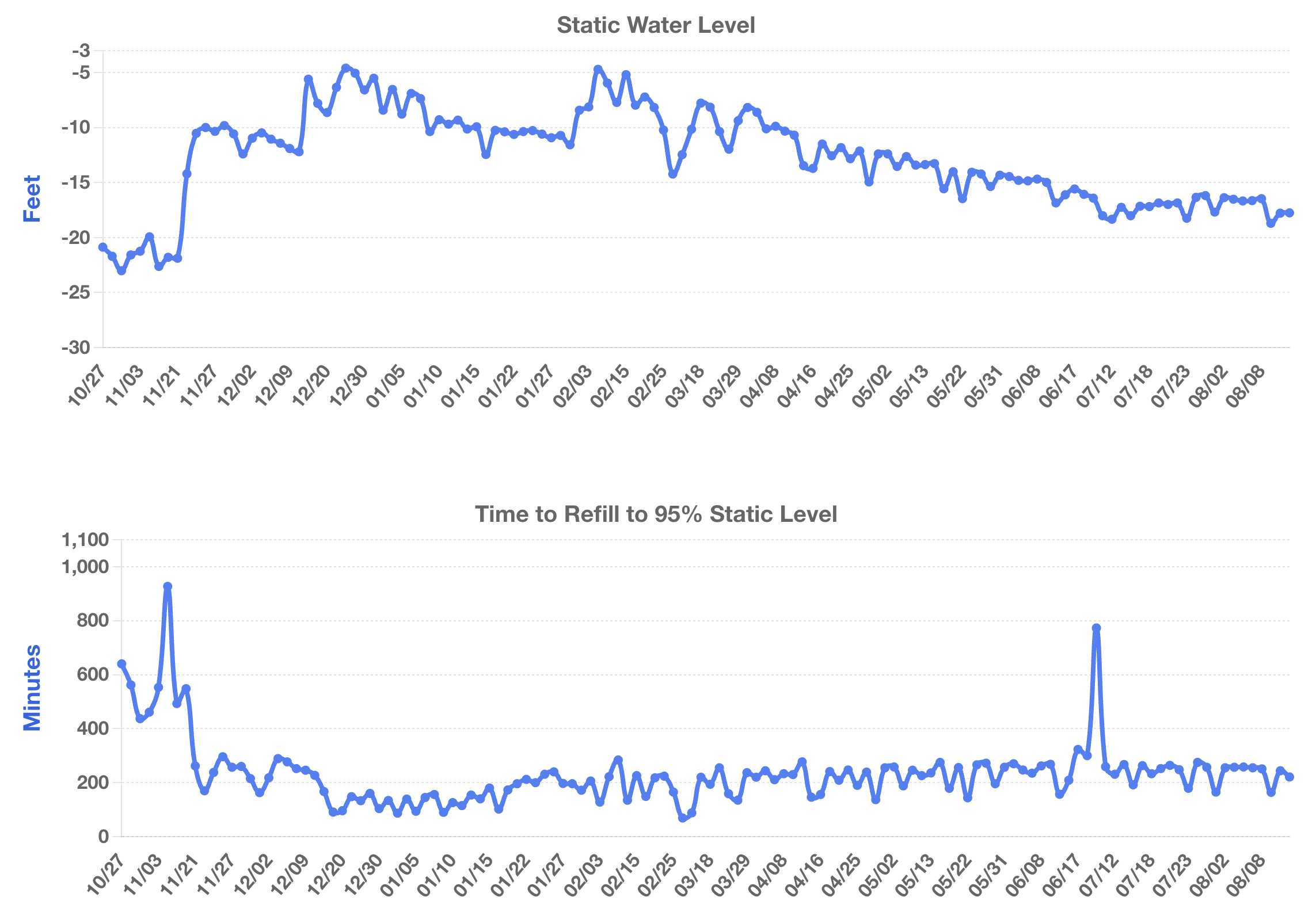
Trends over time:
These graphs show long-term variations in two metrics. Data is for a shallow well in northern California where rainfall patterns are highly seasonal. The period covered starts in the fall at the end of one dry season, goes through a winter rainy season, and then progresses through the summer dry season.
Static water level (SWL)—upper graph:
SWL rises dramatically during multiple rain events during the winter rainy season and then drops down through the dry season.
Well recovery time—lower graph:
Time for well to recover to 95% SWL after CFW ceases. At end of dry season (left side of graph) aquifer level is low and recovery time is long. During rainy season, when aquifer is much higher, recovery time is noticeably shorter.
Long-term trend analysis reveals seasonal patterns and helps predict aquifer behavior throughout the year.
Well/aquifer metrics generated by Cormit for all wells
Time-series (hourly, daily, monthly)
Tracking well and reservoir during CFW cycle:
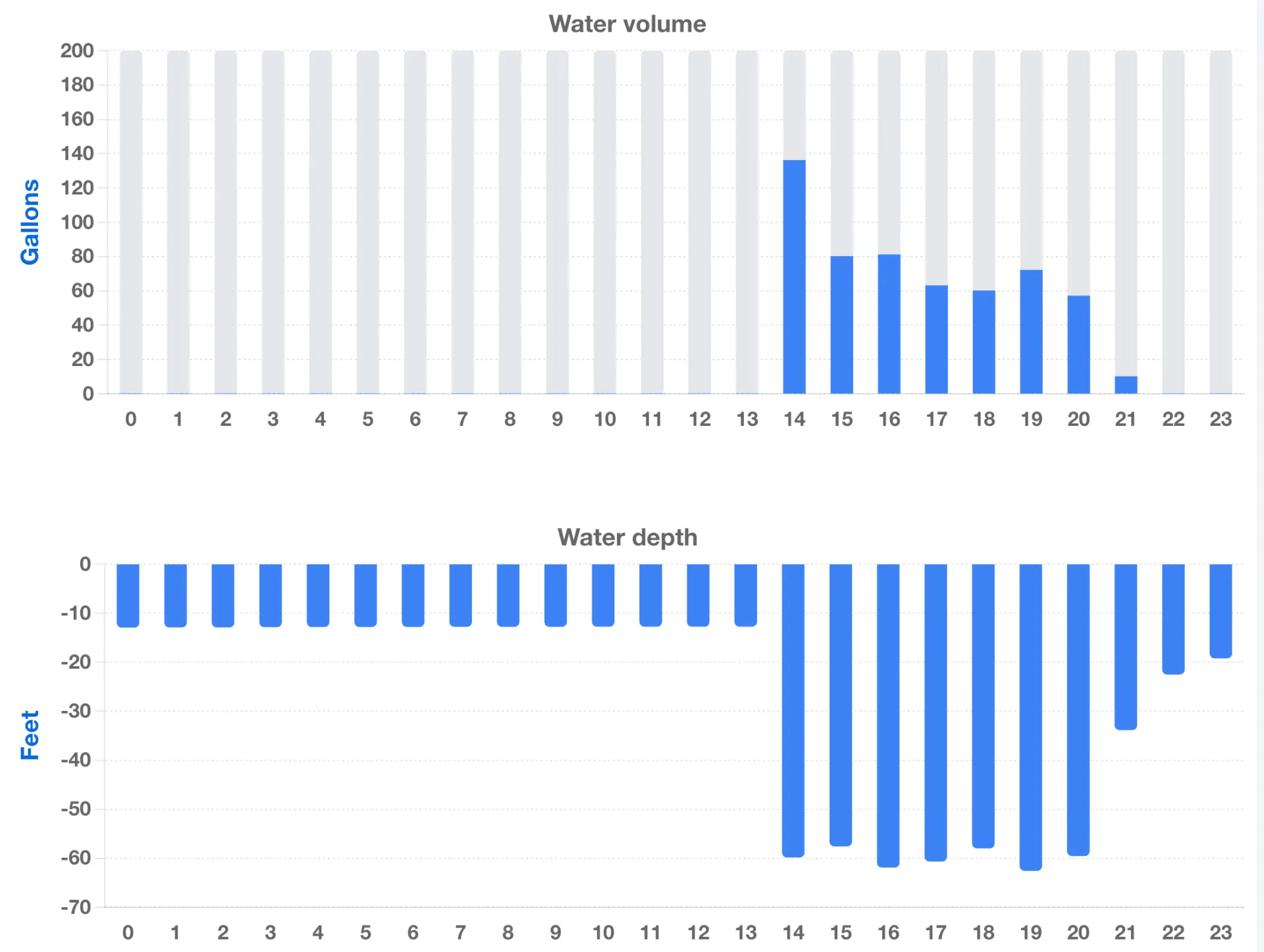
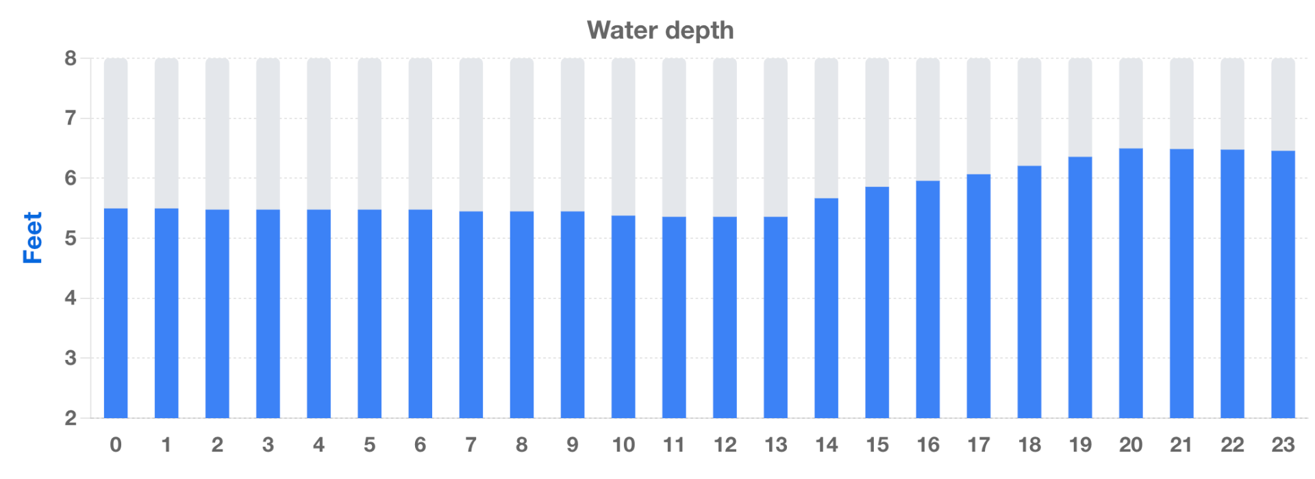
These three graphs show hourly data for well output, water depth in well, and water depth in reservoir over a day when a CFW occurred.
Well output (top graph):
CFW is initiated during hour 14 and continues until hour 21. Well production rate declines over this period.
Water depth in well (middle graph):
Prior to CFW, water depth is at SWL. During CFW cycle, depth drops down almost to the level of the pump as this poorly performing aquifer adds relatively little water to the well in between pump cycles. After CFW, well refills over a period of hours and approaches SWL again.
Water depth in tank (lower graph):
Prior to CFW, level of water in tank drops as reservoir water is consumed. In hour 13, water level in tank has dropped to the trigger point for minimum desired level and CFW begins. In hour 21, water level in reservoir has risen to trigger point for maximum desired water level and CFW ends.
Time-series data provides detailed visibility into the complete well and reservoir system dynamics.